Real-time ray tracing for Digitally Reconstructed Radiograph (DRR) generation

In medical imaging, a Digitally Reconstructed Radiograph (DRR) is a computed radiograph image (2D) produced from volumetric data (3D) via the simulation of the X-ray imaging process. This simulation is known to be already a computationally intense task for a moderate-size dataset due to how X-ray work. I have been working on a (ray-tracer) renderer that generates DRRs in real-time without sacrificing precision. In this post, I will tell you about this exciting project and its results.

X-Ray Imaging

To understand why it is a computationally heavy task, we need to talk a bit about how X-ray imaging works and how it differs from traditional surface rendering. Loosely speaking, surface rendering refers to the imaging process where the light hits a surface, and the light is scattered and reflected toward an observer. This is how the naked eye perceives the environment when visible light reflects from objects.

On the other hand, X-ray radiation can penetrate opaque objects as they are high-energetic electromagnetic radiation (on average, 100 times the energy of sunlight). What we commonly call an "X-Ray" is the image formed by attenuated X-Ray radiation passing through an object. Therefore, the X-ray imaging process is not a local imaging process as a surface-hit interaction but a sum of them.

The whole attenuation process is usually modeled by Lambert's-Beer's Law:

where is the attenuation coefficient and the initial radiation intensity. The integral is along the ray direction and parametrized by the start position and end position .

The attenuation actually depends on the X-Ray's wavelength and the medium's atomic number, mass density, and thickness. Current CT technology effectively stores a monochromatic image. This creates image artifacts, which are sometimes call "beam-hardening" effects. As long as there does not exist a commercial CT machine that produces tomographic images with multiple wavelength channels, Lambert's-Beer law is good enough for the current input data in the general case.

Driving Axis

The data consists of a set of computer tomography slices (usually just called CTs) that stack together to form a volumetric data set. The density values between slices are obtained via interpolation. See figure 1 below. We render the volume by shooting rays from a common source and accumulating the density values. The sum of the collected values allows us to reconstruct a radiograph from the CTs. These computations are all done in the GPU to take advantage of the independence of rays in this process—moreover, rays generated inside a thread group benefit from the coherence of being inside the same bundle.

When a ray intersects the volume, we take ray steps through the driving axis, as shown in figure 2 below. The horizontal lines are the slices, while the vertical lines connect the corresponding pixels in different slices. The driving axis is the axis with the largest ray direction component. Instead of a fixed ray path division, we take ray steps that depend on the number of slices and slice size. The circles in the image below mark the steps. Sampling with the driving axis has two advantages: first, it avoids the bias from small radiological paths when the number of steps is constant (consider intersections close to the corners versus an average intersection!). Second, we reduce the dimension of interpolation by one when estimating the density between slices.

Let's now review the results.

Results

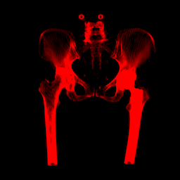
I wrote a compact SwiftUI application for visualizing in real-time the reconstructed radiographs produced by this ray tracer. It achieves a generation of a new DRR every 16.6 ms. Using a CT of a Hip, I obtained this beautiful DRR.

The ray tracer renderer was hardware-accelerated with Metal. Metal (version 3.0) is a C++14-based shading language with extensions and restrictions to the original specification (ISO/IEC JTC1/SC22/WG21 N4431). Although the standard library of Metal provides some ray tracing functionality, I wanted complete control of the intersection routines in the GPU to investigate intersection routines, so I wrote my own custom intersection shaders in the Metal Shading Language (MSL). Of course, one should use as much of the standard library as possible for a final production application. These demos ran on a MacBook Pro M1 with 16 GB of memory. The GPU in the M1 has eight cores with an L1 Cache of 128 KB for instructions and 64 KB for data.

The application has one rotating anatomical view mode (changing from the so-called "coronal" to the "sagittal" views)

Leveraging my fly camera project in a ray tracer, I added another mode where we can freely move to any pose using the mouse or touchpad.

I am quite happy with the results so far and how great Metal is for computing and visualization!